Naive Bayes Is About Asking Questions Your Data Can Answer

Detecting spam messages

The autumn chill wakes Alex up and she loves the amber skies so much. She checks her phone first thing in the morning and sees a new message on Telegram:

Alex immediately recognizes the message as suspicious. But billions of messages are sent every day, and a messaging platform can’t rely on users to identify every scam. How can a computer automatically decide whether a message is spam?

Imagine you’re one of the engineers building Telegram. As responsible engineers, we want to help our users to stay immune and safe from online threats, so we decide to mark shady messages with a spam badge.

We already have a simple database of messages that our colleagues have manually labelled as spam or not spam. Something like:

1
2
3
4
5
6
7
8
9
10
11 +------+-------------------------------------------+-----------+
 | #    | messages                                  | is_spam   |
 +------+-------------------------------------------+-----------+
 |     1| FREE GIFTS! Get your gift from https://...| true      |
 +------+-------------------------------------------+-----------+
 |     2| Heyyyy, wanna hang out today :D           | false     |
 +------+-------------------------------------------+-----------+
 | ...  | ...                                       | ...       |
 +------+-------------------------------------------+-----------+
 |10,000| Transfer $20 to this suspicious account...| true      |
 +------+-------------------------------------------+-----------+
copy
But how do we get an answer for our exact message sent to Alex from this database?
Note
When I use the word database throughout this blog post, I am referring to this research database that has been enriched with is_spam column and not the actual application database.
The question we wish we could answer
We are really interested in finding the answer to this question: Is this message spam or not? Really simple question, but our computers cannot skim through the text and tell us their gut feelings.
To put this question in technical terms we can ask this instead: Is a message spam, if it contained the exact words in order of the original message we saw above? This is more aligned with computers because we have identified a piece of data that a computer can check and give us the answer based on that. We would need an enormous database that maps any possible message to is_spam flag. In Alex’s case, the database needs to have a record like this:
1
2
3
4
5
6
7 +------+-------------------------------------------+-----------+
 |10,001| Hey I found out that you're stuck on the  | true      |
 |      | Bronze ranking in League of Legends game. |           |
 |      | You should totally trust me and give me   |           |
 |      | your password so I can help you!          |           |
 |      | COMPLETELY FREE!                          |           |
 +------+-------------------------------------------+-----------+
copy
As you have probably guessed, this is not feasible. If a message on Telegram can have an average of 4,000 characters, and allows UTF-8 characters, the number of all possible string combinations is astronomical! Having $1,000,000^{4,000}$ records in our database and determining their initial flag value is not possible.
We change our mindset a bit. We give up on answering it by memorizing every possible message. Returning exact answers requires having predefined databases of knowledge for every possible input, which is clearly impossible. So what do we do? The first step is to move towards calculating the most probable answer instead of retrieving exact answers. Answering in terms of probabilities allows us to use mathematics on a smaller set of data and we can estimate the most likely answer based on that. This saves us lots of time and effort.
Compare the two questions and notice the mindset shift:
From: Is a message spam, if it contains the exact words in order of the original message we saw above? which gives us answers of yes and no:
Let Alex’s Message be $M$.
$$f(M) \to {\text{False},\text{True}}$$
To: How probable it is for a message to be spam, if it contains the exact words in order of the original message we saw above? which gives us answers in the range of 0% to 100%:
$$P(\text{Spam} \mid M) \to [0, {100}]$$
Conditional Probabilities Refresher (Part I)
The notation $P(\text{Spam} \mid M)$ might look a little alien at first. It certainly did to me. But don’t worry—it’s much simpler than it looks.
A good way to read the vertical bar (|) is “given that we know…”. So whenever you see:
$P(A \mid B)$
mentally read it as:
“What is the probability of A, given that we know B?”
Let’s make this more tangible.
 Imagine you’re out on your morning walk when you meet your new neighbor. You’d really like to start the conversation by saying “Wind’s howling.” But first you wonder whether they’ve ever played The Witcher 3.
 
Without knowing anything else about them, you can only make a rough guess. Suppose around 80 million people have played the game out of a world population of roughly 8 billion. Then the probability that a random person has played it is about 1%. In mathematical notation, we write this as:
$P(\text{Witcher III Player}) \approx 1\%$
But then you notice something interesting. They’re wearing a wolf medallion—the one Geralt wears throughout the game. Suddenly your estimate changes. You’re no longer asking: “What is the probability that my neighbor has played The Witcher 3?” Instead, you’re asking:
“What is the probability that my neighbor has played The Witcher 3, given that I know they’re wearing a wolf medallion?”
In mathematical notation, that’s simply:
$P(\text{Witcher III Player} \mid \text{Wearing a Wolf Medallion})$
Seeing the medallion doesn’t prove they’ve played the game, but it certainly gives us more confidence. Maybe our estimate jumps from 1% to 90%. That’s all conditional probability is: updating our belief after learning new information.
Hmmm. Changing the question from an exact lookup to a probability certainly helps because we don’t need to have all the message in our database but we can’t still answer this question directly. The attempt to find messages from the database with the same exact words and order will most likely yield nothing. Each message has different words and punctuation.
Deadlock it seems. 😲 Unless…
The question our data can answer
Like in RPG games, when you get stuck on one quest, you leave it alone and complete another one. Sometimes solving a different problem gives you exactly the item you needed for the first. Our first step seems logical but how can we get away with storing all the messages? We are stuck so we start thinking about the questions that we CAN answer based on our little database that we have.
How common are spam messages?
This is a simple question. We query our database and get that answer quickly.
1
2
3
4SELECT COUNT(CASE WHEN is_spam = true THEN 1 END) * 100.0 / COUNT(*)
FROM messages;
# -----------------------------------------
# result: 2%
If Alex gets another message, without looking at its content, we are 2% sure that the message is spam. And this looks awfully the same as this mathematical expression: $P(Spam)$.
If a message is spam, how often does it contain the target message?
Among the posts that are spam, how frequently do we see words that we are looking for (the ones in the original post). In Math language we can show it with $P(M \mid \text{Spam})$.
1
2
3
4
5SELECT COUNT(CASE WHEN
                is_spam = true AND
                message LIKE '%<MESSAGE_TEXT>%' THEN 1 END) * 100.0 /
       COUNT(CASE WHEN is_spam = true)
FROM messages;
In this example, we are searching for the message for its exact text. This will probably return zero. Let this thread stay here, we’ll come back to it.
How often do the messages contain the target message?
What about all the posts? What is the rate of those words appearing? No matter what, we are going to receive messages that contain sus words but they are not sus themselves! (You’re free to substitute the word “sus” with “spam”). This is also equivalent to $P(M)$.
1
2
3SELECT
COUNT(CASE WHEN message LIKE '%<MESSAGE_TEXT>%' THEN 1 END) /
COUNT(*);
Hmmm. This is not going to find anything useful either.
The naive assumption
To be precise, if we want to find out if the message sent to Alex is spam or not, then $P(M \mid \text{Spam})$ translates to “How often spam messages contain the exact string of $M$” and that is probably zero. Each message is different in punctuation, choice of words, names, and everything. The same applies to $P(\text{TEXT})$. We have to do something about them. Conditional independence to the rescue!
Conditional Probabilities Refresher (Part II)
In the last example, wearing a medallion helped us more confident about the neighbor being a Witcher III player. Imagine we want to start the conversation with a Japanese poem and we want to measure our chances if they will understand it fully or will they smile gently and think this is some prank or something. Does him wearing a wolf medallion tell us anything about his understanding of the Japanese language? Probably not,
Knowing they are wearing a wolf medallion is useless information in this case, and we say these two probabilities are independent.
Let:
(J): Comprehending Japanese
 
(M): Wearing a Wolf Medallion
$P(J \mid M) \approx P(J)$
Now let’s do another thought experiment. What is the probability of a coin coming off as heads after flip and a dice turning out as 6 after we roll it, given that we know the weather is rainy.
In mathematical language:
Let:
(C): $\text{Coin} \to \text{heads}$
 
(D): $\text{Dice} \to 6$
 
(R): $\text{Rainy Weather}$
$P((C, D) \mid R)$
Well, we can say for sure that knowing the weather condition is useless information when we want to predict a coin flip and dice roll. We can say they are independent. So we have:
$P(C, D) \to P(C) \cdot P(D) \to P(C \mid R) \cdot P(D \mid R)$
Note that, to get to the final answer, we calculated each probability on its own and multiplied them all together.
We improvise. We assume that once we know the message is spam then each word in the message is independent from the others. In the real world, words are correlated. Seeing the word “send” means there is slightly more chance for the word “password” to be seen in next words. This assumption is why this technique is called 🙂‍↕️
Naive 
. We naively think words are independent but in spam detection this serves us perfectly fine. This assumption turns out to be useful here. Remember this question?
If a message is spam, how often does it contain the target message?
With the newly learned technique, the question translates to:
$$\begin{aligned}
P(M \mid S) &= P(M_0 \mid S) \cdot P(M_1 \mid S) \dots P(M_n \mid S) \\[12pt]
  &= P(\text{Hey} \mid S) \cdot P(\text{Give} \mid S) \dots P(\text{FREE} \mid S)
\end{aligned}$$
Which we can solve with multiple queries! Something like:
1
2
3
4
5SELECT COUNT(CASE WHEN
                is_spam = true AND
                message LIKE '%<MESSAGE_i>%' THEN 1 END) * 100.0 /
       COUNT(CASE WHEN is_spam = true)
FROM messages;
Changing the question
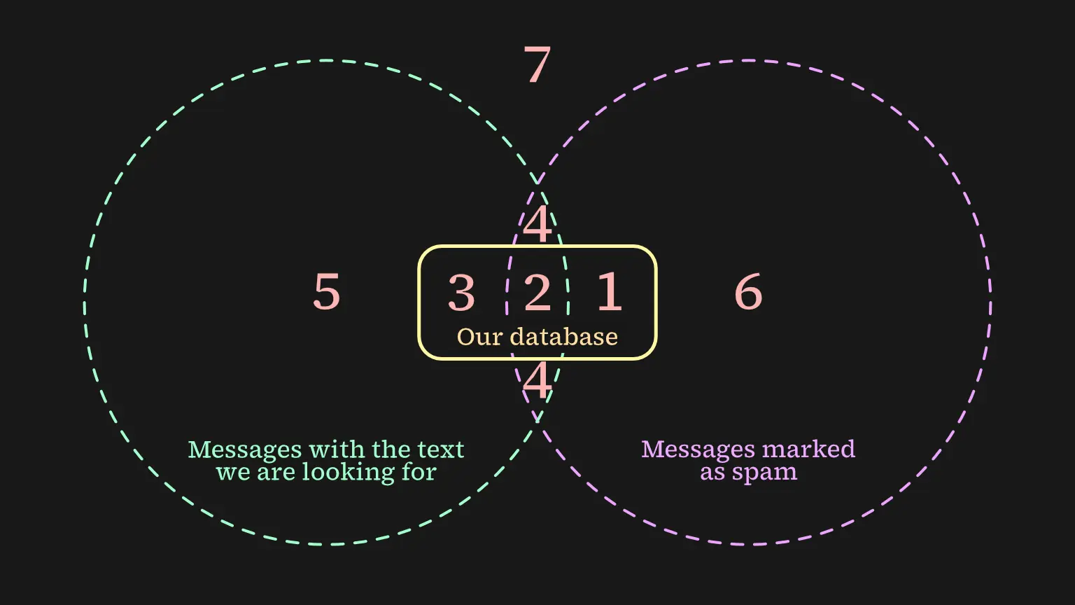
The questions in the previous section seem very random but I had a purpose when I brought them up. What if I told you those random questions will help us answer our main question? Take a look at this diagram:
1 to 7: Any possible message content that can be sent over Telegram
 
1, 2, and 3: Our database that our colleagues have provided. It contains 10,000 messages.
 
$\boldsymbol{\color{#f59e0b}{\dfrac{1,2}{1,2,3}}}$: The amount of spam messages in our database divided by the total number of messages. It answers the question of “How common are spam messages?”.
 
$\boldsymbol{\color{#8b5cf6}{\dfrac{2}{1,2}}}$: A fraction of messages that contain the words we are looking for over all spam messages, all in the scope of our database. It answers the question of “If a message is spam, how often does it contain the message $\bold{M}$?”.
 
$\boldsymbol{\color{#14b8a6}{\dfrac{2,3}{1,2,3}}}$: The proportion of messages containing our target message relative to all messages in our database. It provides an answer to the question, “How often do messages contain the message$\bold{M}$?”.
Now, to answer ”How likely is the message sent to Alex to be spam?”, we can look at the diagram and say $\boldsymbol{{2}/{2,3}}$ looks like the probability we are looking for and that is correct. We can put all the pieces together and reach the Bayes’ theorem ourselves.
The general Bayes’ theorem we’ve been building toward (you saw it at the start of the blog too😅):
$$P(A \mid B) = \dfrac{P(B \mid A) \cdot P(A)}{P(B)}$$
Applied to spam classification:
$$P(\text{SPAM} \mid M) = \dfrac{P(M \mid \text{SPAM}) \cdot P(\text{SPAM})}{P(M)}$$
In words: how likely a message is spam given it is $\bold{M}$ equals how often spam messages contain $\bold{M}$, times how common spam is overall,
divided by how common the message $\bold{M}$ is across all messages.
Now mapping this to our diagram:
$$\begin{aligned}
\dfrac{2}{2,3} &= \dfrac{\color{#8b5cf6}{\dfrac{2}{1,2}} \cdot \color{#f59e0b}{\dfrac{1,2}{1,2,3}}}{\color{#14b8a6}{\dfrac{2,3}{1,2,3}}} \\[24pt]
&= \color{#8b5cf6}{\dfrac{2}{1,2}} \cdot \color{#f59e0b}{\dfrac{1,2}{1,2,3}} \cdot \color{#14b8a6}{\dfrac{1,2,3}{2,3}} \\[12pt]
&= \color{#8b5cf6}{\dfrac{2}{\cancel{1,2}}} \cdot \color{#f59e0b}{\dfrac{\cancel{1,2}}{\cancel{1,2,3}}} \cdot \color{#14b8a6}{\dfrac{\cancel{1,2,3}}{2,3}} \\[12pt]
&= \dfrac{2}{2,3}
\end{aligned}$$
“Wait, what? We found out that the answer to our original question is a simple fraction that we could have found since the dawn of this blog post but why did we go through answering random questions and proving that doing math with them will get us to the very same answer?” you might ask, and I appreciate your attention to the things we have done.
Let’s make things more clear.
Posterior: $\bold{\dfrac{2}{2,3}\equiv P(\bold{Spam} \mid M)}$
The diagram gives us the illusion that we could have found the start from the very start. Let’s review it one more time. We are searching for $P(\text{Spam} \mid M)$. We can’t directly calculate $P(\text{Spam} \mid M)$ unless we have a database that stores all the messages with their labels, which is exactly what we’ve been trying to avoid.
Why not use the naive technique here and tokenize the $\bold{M}$ so we don’t have to match an exact message? Well, that doesn’t make sense. We proved we can use the technique on $A$ when the expression is like: $P(A \mid B)$, where $B$ is independent. The other way around is not valid.
Likelihood: $\bold{\color{#8b5cf6}{\dfrac{2}{1,2}\equiv P(M \mid \bold{Spam})}}$
Once we know the message is spam, we assumed that each word appears independently of the others. This lets us estimate $P(M \mid \text{Spam})$ by multiplying the probabilities of the individual words.
Prior: $\bold{\color{#f59e0b}{\dfrac{1,2}{1,2,3}\equiv P(\bold{Spam})}}$
We calculate the overall number of spam messages. Simple. No tricks.
Denominator: $\bold{\color{#14b8a6}{\dfrac{2,3}{1,2,3}\equiv P(M)}}$
We didn’t talk about this part of the formula too much. The reality is we can’t directly calculate this part in a way that we mean it. Searching for exact matches of the message $M$ will probably return zero, which would make our effort meaningless.
Practical implementations usually omit this denominator because it is identical for every class being compared. These implementations also calculate the not spam equivalent part of the formula and whichever returns a higher score, that label gets elected.
$$\begin{aligned}
P(\text{Spam} \mid M) &\lesseqqgtr P(\text{Not Spam} \mid M) \\[12pt]
P(M \mid \text{Spam}) \cdot P(Spam) &\lesseqqgtr P(M \mid \text{Not Spam}) \cdot P(Not Spam)
\end{aligned}$$

History

Thomas Bayes was a man going about his life in the 18th century, and he knew nothing of digital minions and them learning the ways of humans. Okay, I should stop with the 18th century prose writing. He was a minister, statistician, and philosopher and he was trying to answer a question:

Suppose I believe something is true about the world. Then I observe new evidence. How should I, a rational person, change my beliefs?

For almost two centuries, Bayes’ theorem remained mostly a tool for statistics and philosophy and for many years Bayesian methods were overshadowed by frequentist statistics. In the twentieth century, computer scientists realized that many machine learning problems have exactly the same structure. Although the applications changed dramatically, the underlying mindset remained exactly the same: observe evidence, then update your beliefs.

Where the trick breaks down

One of the assumptions we made throughout this article was that the words in a message behave independently once we know whether the message is spam or not. This assumption is obviously not true. Words often appear together and influence one another. Surprisingly, despite being wrong, the assumption works well enough for many text-based classification tasks.

However, there are situations where this simplification breaks down completely. Consider medical image classification. Imagine we want to answer the following question: Given this X-ray image, how likely is it that the patient has cancer?

We would like to find an answer for:

by calculating this expression:

Everything looks similar. The issue starts when we try to apply the naive technique. The naive approach would assume each pixel is an independent piece of data:

But images don’t work that way. Pixels of an image are highly correlated, to the point that our independence assumption breaks down. Each pixel has neighboring pixels which are very likely to have similar color values. Edges, color contrasts, and features of medical images all are made from groups of highly correlated pixels. The naive technique throws away all of these important pieces of information and that’s why it can’t answer correctly in this case.

In other words, Naive Bayes is an excellent algorithm when the independence assumption is a reasonable approximation, such as spam filtering or simple document classification. But when the features are highly correlated—as in images, audio, or videos—the assumption becomes too unrealistic, and more expressive models are usually preferred.

Wrap up

When we started this article, our question was very simple:

Is Alex’s message spam?

The easiest solution was to search for that exact message in a database, but we quickly discovered why that approach could never work. There are simply too many possible messages.

Instead of concluding that our data couldn’t answer the question, we changed the question into several smaller ones that it could answer:

• How common is spam?
• How often do spam messages contain these words?
• How often do messages in general contain these words?

Once we had answers to those questions, Bayes’ theorem wasn’t a random formula anymore. We reverse-engineered the formula by answering simpler questions that our data actually could answer.

The “naive” part came from one bold assumption. Once we know the label, we pretend the features are independent. That assumption isn’t true in reality, but for many text based classification problems it is good enough to produce surprisingly strong results.

Perhaps that is the biggest lesson behind Naive Bayes. Machine learning is not always about finding the perfect model. Sometimes it is about asking questions that your data is actually capable of answering.